| Author | Jingyi Wang |
| Module | INT104 |
| Teacher | Xiaobo Jin |
| Date | Apr. 27, 2021 |
1. Introduction
Text categorization is used to classify a set of documents into categories from known labels. To complete the text classification, the documents need to be transformed into a vector space model first. The dimension of the vector is the number of all non-repeating words that occur in all documents. In this lab session, I will firstly pre-process the documents, including spliting, removing stopwords and stemming. Then I will generate a frequency array against each unique word in each document. After that, calculate tfidf-weighting and tfc-weighting. Finally I will visualize the result array by t-SNE method to evaluate the vector space model.
2. Design and Implementation
2.1 Preprocessing
a. Read Stopwords
In this block, the stopwords are read from “stopwords.txt”. Then a set called stopwords_set is initialized from the list of stopwords. (20 marks)
# Init stopwords set from "./stopwords.txt"
with open("stopwords.txt", "r", encoding='Latin1') as stopwords_file:
    stopwords_set = set(stopwords_file.read().split())
b. Data Structure in Preprocessing
word_count_all_docs is a nested list. Its length is the number of documents. Each row in this nested list is also a list, which stores the occur times of each unique word.
The lengths of rows of word_count_all_docs are different and incremental, since after the first few of documents are processed, there are only hundreds of unique words. But after all of the documents are processed, there will be about 28000 unique words.
# The number of rows will be the number of documents,
# and numbers in each row are words' occur times for each document.
word_count_all_docs = list()
word_index is a dictionary, used to look up the index of each unique word quickly. Keys in it are all of the unique words, and values are 0, 1, 2, ..., (N_words-1). For example, assume there are four unique words in all of the documents, word_index looks like this:
Keys: ["we", "love", "computer", "science"]
Values: [0, 1, 2, 3]
# Keys are all of the unique words,
# values is an increasing series, i.e., [0, 1, 2, ..., (N_words-1)]
word_index = dict()
num_documents_per_category is used to store the names and numbers for each category. These data will be used in training and ploting. Content is:
Keys: ['alt.atheism', 'comp.graphics', 'rec.motorcycles', 'soc.religion.christian', 'talk.politics.misc']
Values: [480, 584, 598, 599, 465]
# Keys are names of five categories,
# values are five numbers of documents for corresponding categories.
num_documents_per_category = dict()
c. Read Dataset, Perform Word Stemming and Update Counter
Read dataset files, Delete non-alphabet letters
In line 2-5 of the following code block, I scanned all of the subdirectories in “dataset” folder. In each subdirectory, scan and open every text file, then split the words into a list, shown in line 8-12. (20 marks)
Perform word stemming
I used stemmer = SnowballStemmer("english") object to extract the word stem. In line 27, after the words are converted to lowercase with non-alphabet letters removed, word stemming algorithm is performed. The reason I chose Snowball Stemmer over Porter Stemmer is that Snowball Stemmer has better performance according to the docs of nltk [1]. (20 marks)
Update word counter and word index
After a word has been lowercased, non-alphabet-letters removed and stmmmed, we will check whether it is a new unique word, i.e., whether this word is in word_index.keys().
If it is a new unique word, we add it in word_index dictionary, and append counter 1 to the list of currnet row. If this unique word is exist, we update the counter list of current row.
Here is the code block for 3 steps above:
# Iterate through each series (subdirectory)
for subdirectory in os.listdir("dataset"):
    path = "dataset/" + subdirectory + "/"
    num_documents_per_category[subdirectory] = 0
    print(elapsed_time(), "Detected category: " + subdirectory + ", reading data files...")

    # Iterate through each document in current subdir
    for filename in os.listdir(path):
        num_documents_per_category[subdirectory] += 1
        with codecs.open(path + filename, 'r', encoding='Latin1') as file:
            # Create a list of raw words
            raw_words = file.read().split()
        # Init an empty list with length of currently found unique words
        word_count_current_doc = [0] * len(word_index)

        # Iterate through each raw words in this document
        for word in raw_words:
            # Skip stopwords
            if word.lower() in stopwords_set:
                continue
            # Remove non-alphabet letters
            formatted_word = re.sub(r'[^a-z]', '', word.lower()).strip()
            # Skip empty words or single letter
            if len(formatted_word) < 2:
                continue
            # Run stem extraction
            word_stem = stemmer.stem(formatted_word)
            # Check whether current word has been added in word_index
            if not (word_stem in word_index):
                # Update the dict of word_index: {key: word, value: len(word_index)}
                word_index[word_stem] = len(word_index)
                # Append the current counter with 1
                word_count_current_doc.append(1)
            else:
                # Add 1 to the current counter
                word_count_current_doc[word_index[word_stem]] += 1
        # Add the counter of current document into the nested list
        word_count_all_docs.append(word_count_current_doc)
Finally, print out the total numbers of unique words and documents.
N_words = len(word_index)
N_docs = len(word_count_all_docs)
print(elapsed_time(), N_docs, "documents have been read,",
      N_words, "unique words are detected. Generating numpy array...")
2.2 TFIDF Representation
A well known approach for computing word weights is the TFIDF weighting [2], which assigns the weight to word i in document k in proportion to the number of occurrences of the word in the document, and in inverse proportion to the number of documents in the collection for which the word occurs at least once: \[ a_{ik}=f_{ik}*\log(\frac{N}{n_k}) \] where \(f_{ik}\) is the frequency of word k in document i, and \(n_k\) is the total number of times word k occurs in the dataset.
Convert the Nested List to Numpy Array
After we counted the occur times for each unique word in each document, and stored the result in nested list word_count_all_docs, we need to convert it to numpy array for the convenience of later calculations.
As mentioned above, the lengths of rows of word_count_all_docs are increasing. So we fill each line of data to the left of each line of the numpy array, and fill the extra space on the right with zeros, if len(word_count_all_docs[i]) < N_words in i-th row. (10 marks)
# Create a numpy array with known shape: [N_words, N_docs],
weight_array = np.zeros([N_docs, N_words])
for i in range(0, N_docs):
    # Fill each row of numpy array with the counter of each document
    weight_array[i][0:len(word_count_all_docs[i])] = word_count_all_docs[i]
print(elapsed_time(), "Numpy array is generated. TFIDF representing...")
Calculate nk: Numbers of Documents Contain Word k
According to TFIDF formula, we can calculate the sum of all rows of frequency array to get \(n_k\). The result is one row, represents the total number of occurrences of each unique word in all documents. (10 marks)
# Sum of all of the rows, i.e., sum word occur times for each word
n_docs_contain_each_word = weight_array.clip(0, 1).sum(axis=0)
Calculate fik: Term Frequency of the Words in each Document
Divide the occur times of each unique word in a document by the total number of words in this document:
# Convert number of occurs to term frequency (TF)
weight_array /= weight_array.sum(axis=1).reshape([N_docs, 1])
Perform TFIDF Representation
Firstly we calculated a row of factor, IDF, which is equal to: \(\log(\frac{N}{n_k})\) :
# Inverse Document Frequency (IDF)
idf = np.log10(N_docs/n_docs_contain_each_word).reshape([1, N_words])
Then multiply each row in the current weight array (TF), by the row of factor above:
# Convert term frequency to TFIDF result
weight_array *= idf
TFC-Weighting: Normalize the Representation of the Document
We do not want the calculated TFIDF weights to be affected by the length of the document because of the different document lengths. Therefore we should consider dividing the TFIDF weights by a value related to the length of each document. This method is called tfc-weighting [3], given by: \[A_{ik}=\frac{a_{ik}}{\sqrt{\sum_{j=1}^{D}a^{2}_{ij}}}\]
# Normalize the representation of the document
weight_array /= np.sqrt(np.sum(weight_array**2, axis=1)).reshape([N_docs, 1])
Save the Numpy Array
Finally, we can save this numpy array of calculated weight into a file:
# Save TFIDF array file and print out the file size.
np.savez('train-20ng.npz', X=weight_array)
size = os.path.getsize('train-20ng.npz') / 1024.0**2
print(elapsed_time(), "Saved into 'train-20ng.npz', size:", round(size, 2), "MB.")
3. Test and Data Visualization
3.1 Time Consumption
Following code is used to record the start timestamp and generate a string to show elasped time:
# Record start time for performance status
start = time.time()
# Return a string contains elapsed time from start
def elapsed_time():
    return '(' + str(round(time.time() - start, 2)) + 's)'
Then, to test whether my feature generation algorithm works, and to see how long it takes for each step. Printed out messages are shown below:
C:\Users\kexue\Desktop\INT104\Assignment2\venv\Scripts\python.exe C:/Users/kexue/Desktop/INT104/Assignment2/Assignment2.py
 (0.0s) Detected category: alt.atheism, reading data files…
 (1.57s) Detected category: comp.graphics, reading data files…
 (3.06s) Detected category: rec.motorcycles, reading data files…
 (4.43s) Detected category: soc.religion.christian, reading data files…
 (6.56s) Detected category: talk.politics.misc, reading data files…
 (8.59s) 2726 documents have been read, 27979 unique words are detected. Generating numpy array…
 (10.96s) Numpy array is generated. TFIDF representing…
 (11.44s) TFIDF array has been calculated.
 (12.57s) Saved into 'train-20ng.npz', size: 581.9 MB.
 ------Feature Generation Done! Visualizing data…------
 (12.82s) T-SNE performing…
 (42.05s) T-SNE completed, plotting…
 (42.46s) T-SNE plot has been saved into 'tsne.png'.
 (94.54s) TFIDF weight plot has been saved into '3.png'.
 (113.24s) Frequency plot has been saved into '2.png'.
 ------All Done! Have Fun!------
 Process finished with exit code 0
We can see it costs about 10 seconds to do the preprocessing part, including reading dataset, stemming, generating frequency array. Then, the calculation of TDIDF weights is a rapid process with the help of numpy, about 0.5s. Average time cost of feature generation process is about 13 seconds. (My CPU is: Intel i5-6200U 2.4GHz)
3.2 Data Visualization: Frequency Array
After the preprocessing, we can plot a scatter plot of the number of occurrences against each unique word in each document by using following code:
# Plot occur frequency against unique words and documents
fig = plt.figure(figsize=(45, 30))
ax = fig.add_subplot(111, projection='3d')
x_axis.clear()
y_axis.clear()
z_axis.clear()
y = 0
for category in num_documents_per_category:
    for nums in range(0, num_documents_per_category[category]):
        for x in range(0, len(word_count_all_docs[y])):
            if word_count_all_docs[y][x] > 0:
                x_axis.append(x)
                y_axis.append(y)
                z_axis.append(word_count_all_docs[y][x])
        y += 1
    ax.scatter(x_axis, y_axis, z_axis, label=category, s=z_axis)
    x_axis.clear()
    y_axis.clear()
    z_axis.clear()
ax.set_xlabel("Words")
ax.set_ylabel("Documents")
ax.set_zlabel("Occur Times")
ax.legend(loc="best")
plt.savefig("2.png")
print(elapsed_time(), "Frequency plot has been saved into '2.png'.")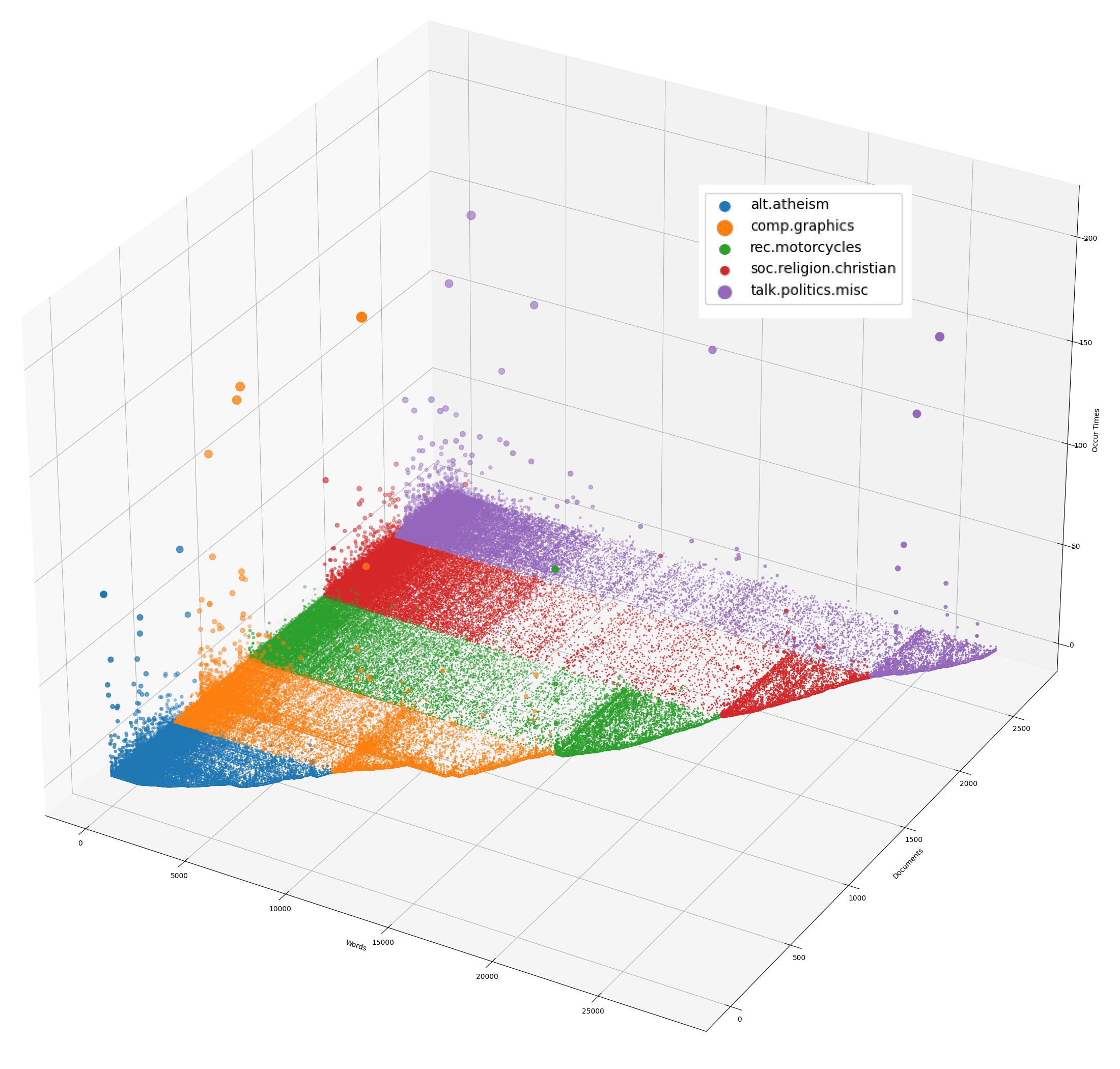
From the figure, it is observed that for each category, there is a region where the current category is more dense and the other categories are not, and it can be guessed that the words in these regions are likely to be more relevant to the topic of the current category.
But for the first few hundred words that appear to occur more often in each category, these words may have less dependence on a specific category.
3.3 Data Visualization: TFC Weight
Use following code to plot the calculated tfc-weight against each unique word in each document:
# Plot tfc-weighting against unique words and documents
fig = plt.figure(figsize=(45, 30))
ax = fig.add_subplot(111, projection='3d')
x_axis = list()
y_axis = list()
z_axis = list()
y = 0
for category in num_documents_per_category:
    for nums in range(0, num_documents_per_category[category]):
        for x in range(0, N_words):
            if weight_array[y][x] > 0:
                x_axis.append(x)
                y_axis.append(y)
                z_axis.append(weight_array[y][x])
        y += 1
    ax.scatter(x_axis, y_axis, z_axis, label=category, s=1)
    x_axis.clear()
    y_axis.clear()
    z_axis.clear()
ax.set_xlabel("Words")
ax.set_ylabel("Documents")
ax.set_zlabel("TFIDF Weight")
ax.legend(loc="best")
plt.savefig("3.png")
print(elapsed_time(), "TFIDF weight plot has been saved into '3.png'.")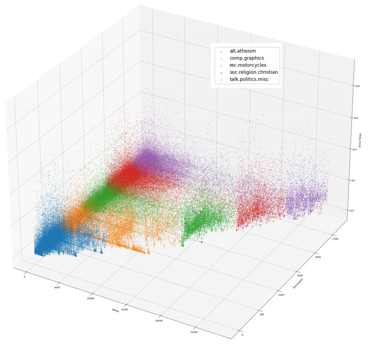
From the figure we see that the dense, high weight regions are basically the same as in Figure 3.2. The difference is that after TFIDF representation, the weight values are mapped to a more reasonable interval, and the extreme data are not obvious anymore.
3.4 Data Visualization: t-SNE Dimension Reduction
t-SNE is a tool to visualize high-dimensional data [4]. It can transform high-dimensional data into 2D or 3D. Using following code with TSNE lib in Sklearn to perform dimension reduction:
# t-SNE reduce dimension
print(elapsed_time(), "T-SNE performing...")
tsne = TSNE(n_components=2)
tsne.fit_transform(weight_array)
tsne_result = tsne.embedding_
print(elapsed_time(), "T-SNE completed, plotting...")
Afterwards, plot the position of each document on the 2D plane as a scatter plot, and use different colors to distinguish between different categories of documents.
# Plot t-SNE result
fig = plt.figure(figsize=(7, 5))
ax = fig.add_subplot(111)
cur = 0
for category in num_documents_per_category:
    x_axis = list(tsne_result[cur:cur+num_documents_per_category[category], 0])
    y_axis = list(tsne_result[cur:cur+num_documents_per_category[category], 1])
    ax.scatter(x_axis, y_axis, label=category, s=3)
    cur += num_documents_per_category[category]
ax.set_xlabel("X")
ax.set_ylabel("Y")
ax.legend(loc="best")
plt.savefig("tsne.png")
print(elapsed_time(), "T-SNE plot has been saved into 'tsne.png'.")
Output plot:
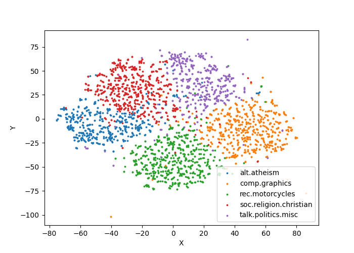
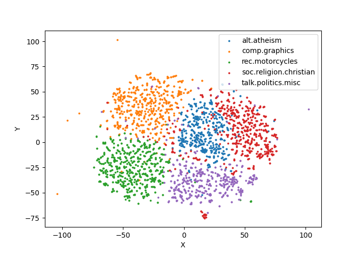
Observe from the figure that the different categories of documents have been almost correctly distinguished.
4. Conclusion
In this lab session, I learned some basic methods and skills to do feature generation, such as stop words set, word stemming, and using python and numpy to generate a vector space model. Afterwards, tfidf weighting and tfc-weighting are calculated as the generated feature.
This report also evaluated the time consumption of each processing step, and then evaluated the vector space model by visualizing data, including raw frequency, tfc-weighting and deduced dimensional model. From the results, we can see that the documents of the same category are clustered together, indicating that we have successfully extracted the features of different categories of documents.
The future work could be dimensionality reduction, since there are still some noise words can be observed from Fig. 3.2. Some methods [5] are used to remove noninformative words from documents in order to improve categorisation eectiveness and reduce computational complexity.
Reference
- [1]“Stemmers,” Natural Language Toolkit — NLTK 3.6.2 documentation, Apr. 20, 2021. https://www.nltk.org/howto/stem.html (accessed Apr. 27, 2021).
- [2]G. Salton and M. J. McGill, Introduction to Modern Information Retrieval. USA: McGraw-Hill, Inc., 1986.
- [3]G. Salton and C. Buckley, “Term-weighting approaches in automatic text retrieval,” Information Processing & Management, pp. 513–523, Jan. 1988, doi: 10.1016/0306-4573(88)90021-0.
- [4]Laurens van der Maaten and G. Hinton, “Visualizing Data using t-SNE,” Journal of Machine Learning Research, vol. 9. pp. 2579–2605, 2008, [Online]. Available: http://jmlr.org/papers/v9/vandermaaten08a.html.
- [5]K. Aas and L. Eikvil, “Text Categorisation: A Survey,” 1999.